Getting Started with Axon

Source

This notebook is copied from this article by Sean Moriarity: https://dockyard.com/blog/2022/01/11/getting-started-with-axon

Preface

NOTE: Before reading, I highly recommending checking out my first post which serves as an introduction to Nx and the Nx ecosystem: https://dockyard.com/blog/2021/04/08/up-and-running-nx

This XKCD was published in September of 2014, roughly two years following deep learning’s watershed moment - AlexNet. At the time, deep learning was still in it’s nascent stages, and classifying images of “bird or no bird” might have seemed like an impossible task. Today, thanks to neural networks, we can “solve” this task in roughly 30 minutes - which is precisely what we’ll do with Elixir and Axon.

NOTE: To say the problem of computer vision is “solved” is debatable. While we’re able to achieve incredible performance on image classification, image segmentation, object detection, etc., there are still many open problems in the field. Models still fail in hilarious ways. In this context, “solved” really means suitable accuracy for the purposes of this demonstration.

Introduction

Axon is a library for creating neural networks for the Elixir programming language. The library is built entirely on top of Nx, which means it can be combined with compilers such as EXLA to accelerate programs with “just-in-time” (JIT) compilation to the CPU, GPU, or TPU. What does that actually mean? Somebody has taken care of the hardwork for us! In order to take advantage of our hardware, we need optimized and specialized kernels. Fortunately, Nx and EXLA will take care of generating these kernels for us (by delegating them to another compiler). We can focus on our high-level implementation, and not the low-level details.

You don’t need to understand the intricacies of GPU programming or optimized mathematical routines to train real and practical neural networks.

What is a neural network?

A neural network is really just a function which maps inputs to outputs:

• Pictures of cats and dogs -> Label cat or dog
• Lot size, square footage, # of bedrooms, # of bathrooms -> Housing Price
• Movie Review -> positive or negative rating

The “magic” is what happens during the transformation of input data to output label. Imagine a cohesive team of engineers solving problems. Each engineer brings their own unique perspective to a problem, applies their expertise, and their efforts are coordinated with the group in a meaningful way to deliver an excellent product. This coordinated effort is analagous to the coordinated effort of layers in a neural network. Each layer learns it’s own representation of the input data, which is then given to the next layer, and the next layer, and so on until we’re left with a meaningful representation: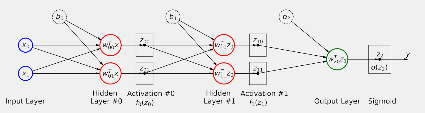

In the diagram above, you’ll notice that information flows forward. Occasionally, you’ll hear the term feed-forward networks which is derived from the fact that information flows forward in a neural network.

Successive transformations in a neural network are typically referred to as layers. Mathematically, a layer is just a function:

$$ f(x; \theta) = f^{(1)}(f^{(2)}(x; \theta); \theta) $$

Where $f^{(1)}$ and $f^{(2)}$ are layers. For those who like to read code more than equations, the transformations essentially boil down to the following Elixir code:

def f(x, parameters) do
  x
  |> f_2(parameters)
  |> f_1(parameters)
end
def f_1(x, parameters) do
  {w1, b1, _, _} = parameters
  x * w1 + b1
end
def f_2(x, parameters) do
  {_, _, w2, b2} = parameters
  x * w2 + b2
end

In the diagram, you’ll also notice the term activation function. Activation functions are nonlinear element-wise functions which scale layer outputs. You can think of them as “activating” or highlighting important information as it propagates through the network. With activation functions, our simple two layer neural network starts to look something like:

def f(x, parameters) do
  x
  |> f_2(parameters)
  |> activation_2()
  |> f_1(parameters)
  |> activation_1()
end
def f_1(x, parameters) do
  {w1, b1, _, _} = parameters
  x * w1 + b1
end
def activation_1(x) do
  sigmoid(x)
end
def f_2(x, parameters) do
  {_, _, w2, b2} = parameters
  x * w2 + b2
end
def activation_2(x) do
  sigmoid(x)
end

The “learning” in “deep learning” comes in learning parameters defined in the above functions which effectively solve a given task. As noted in the beginning of this post, “solve” is a relative term. Neural networks trained on separate tasks will have entirely different success criteria.

The learning process is commonly referred to as training. Neural networks are typically trained using gradient descent. Gradient descent optimizes the parameters of a neural network to minimize a loss function. A loss function is essentially the success criteria you define for your problem.

Given a task, we can essentially boil down the process of creating and training neural networks to:

1. Gather, explore, normalize the data
2. Define the model
3. Define success criteria (loss function)
4. Define the training process (optimizer)
5. Instrument with metrics, logging, etc.
6. Go!

Axon makes steps 2-6 quick and easy - so much so that most of your time should be spent on step 1 with the data. For the rest of this post, we’ll walk through an example workflow in Axon, and see how easy it is to create and train a neural network from scratch.

Requirements

To start, we’ll need to install some prerequisites. For this example, we’ll use Axon, Nx, and EXLA to take care of our data processing and neural network training. We’ll use Flow for creating a simple IO input pipeline. Pixel will help us decode our raw JPEGs and PNGs to tensors. Finally, Kino will allow us to render some of our data for analysis.

Additionally, we’ll set the default Defn compiler to EXLA. This will ensure all of our functions in Axon run using the XLA compiler. This really just means they’ll run much faster than they would in pure Elixir.

Mix.install([
  {:axon, "~> 0.1.0-dev", github: "elixir-nx/axon"},
  {:exla, "~> 0.1.0-dev", github: "elixir-nx/nx", sparse: "exla"},
  {:nx, "~> 0.1.0-dev", github: "elixir-nx/nx", sparse: "nx", override: true},
  {:flow, "~> 1.1.0"},
  {:pixels, "~> 0.2.0"},
  {:kino, "~> 0.3.1"}
])

Nx.Defn.default_options(compiler: EXLA)

The Data

Our goal is to differentiate between images of birds and not birds. While in a practical setting we’d probably want to include images of nature and other settings birds are found in for our negative examples, in this example we’ll use pictures of cats. Cats are definitely not birds.

For images of birds, we’ll use Caltech-UCSD Birds 2011 which is an open-source dataset consisting of around 11k images of various birds. For images of cats, we’ll use Cats vs. Dogs which is a dataset consisting of around 25k images of cats and dogs. The rest of this post will assume this data is downloaded locally.

Let’s start by getting an idea of what we’re working with:

cats = "PetImages/Cat/*.jpg"
birds = "CUB_200_2011/images/*/*.jpg"

num_cats =
  cats
  |> Path.wildcard()
  |> Enum.count()

num_birds =
  birds
  |> Path.wildcard()
  |> Enum.count()

IO.write("Number of cats: #{num_cats}, Number of birds: #{num_birds}")

Fortunately, our dataset is relatively balanced. In total we have around 25000 images. This is a little on the low side for most practical deep learning problems. Both data quantity and data quality have a large impact on the performance of your neural networks. For our example here the data will suffice, but for practical purposes you’d want to conduct a full data exploration and analysis before diving in.

We can use Kino to get an idea of what examples in our dataset look like:

cats
|> Path.wildcard()
|> Enum.random()
|> File.read!()
|> Kino.Image.new("image/jpeg")

birds
|> Path.wildcard()
|> Enum.random()
|> File.read!()
|> Kino.Image.new("image/jpeg")

One thing you might notice is that our images are not normalized in terms of height and width. Axon requires all images to have the same height, width, and number of color channels. In order to train and run our neural network, we’ll need to process each image into the same dimensions.

Additionally, our images are encoded as PNGs and JPEGs. Axon only works with tensors, so we’ll need to read each image into a tensor before we can use it. We can do this using Pixel and a sprinkle of Nx. First, let’s see how we can go from image to tensor:

{:ok, image} =
  cats
  |> Path.wildcard()
  |> Enum.random()
  |> Pixels.read_file()

%{data: data, height: height, width: width} = image

data
|> Nx.from_binary({:u, 8})
|> Nx.reshape({4, height, width}, names: [:channels, :height, :width])

Nx encodes images as values at each pixel. By default, Pixels decodes images in RGBA format. So, for each pixel in an image with shape {height, width}, we have 4 8-bit integer values: red, green, blue, and alpha (opacity). Pixels conveniently gives us a binary of pixel data, and the height and width of the image. So we can create a tensor using Nx.from_binary/2 and then reshape to the correct input shape using Nx.reshape/2.

When working with images, it’s common to normalize pixel values to fall between 0 and 1. This helps stabilize the training of neural networks (most parameters are initialized to a value between 0 and 0.06). To do this, we can simply divide our image by 255:

data
|> Nx.from_binary({:u, 8})
|> Nx.reshape({4, height, width}, names: [:channels, :height, :width])
|> Nx.divide(255.0)

Now, let’s take some of this exploration and turn it into a legitimate input pipeline.

Input Pipeline

Now that we know how to get a tensor from an image, we can go about constructing the input pipeline. In this example, our pipeline will just be an Elixir Stream. In most machine learning applications, datasets will be too large to load entirely in to memory. Instead, we want to construct an efficient pipeline of data preprocessing and normalization which runs in parallel with model training. For example, we can train our models entirely on the GPU, and process new data at the same time on the CPU.

Right now, we can retreive our data as paths to separate image directories. We’ll start by labeling images in respective directories, shuffling the input data, and then splitting it into train, validation, and test sets:

cats_path_and_label =
  cats
  |> Path.wildcard()
  |> Enum.map(&{&1, 0})

birds_path_and_label =
  birds
  |> Path.wildcard()
  |> Enum.map(&{&1, 1})

image_path_and_label = cats_path_and_label ++ birds_path_and_label
num_examples = Enum.count(image_path_and_label)
num_train = floor(0.8 * num_examples)
num_val = floor(0.2 * num_train)

{train, test} =
  image_path_and_label
  |> Enum.shuffle()
  |> Enum.split(num_train)

{val, train} =
  train
  |> Enum.split(num_val)

This sort of dataset division is common when training neural networks. Each separate dataset serves a separate purpose:

• Train set - consists of examples that the network explicitly trains on. This should be the largest portion of your dataset. Typically 70-90% depending on dataset size.
• Validation set - consists of examples that are used to evaluate the model during training. They provide a means of monitoring the model for overfitting as the examples in the validation set are not explicitly trained on. Typically is a small percentage of the train set.
• Test set - consists of examples which are unseen during training and validation which are used to validate the trained model’s performance.

As you’ll see, Axon makes it easy to create a training and evaluation pipelines which make use of all of these datasets.

Next, we’ll create a function which returns a stream given a list of image paths and labels. Our stream should:

1. Parse the given image path into a tensor or filter bad images
2. Pad or crop image to a fixed size
3. Rescale the image pixel values between 0 and 1
4. Batch input images

A batch is just a collection of training examples. In theory, we’d want to update a neural network’s parameters using the gradient of each parameter with respect to the model’s loss over the entire training dataset. In reality, most datasets are far too large for this. Instead, we update models incrementally on batches of training data. One full pass of batches through the entire dataset is called an epoch.

In this example, we’ll batch images into batches of 32. The choice of batch size is arbitrary; however, it’s common to use batch sizes which are multiples of 32, e.g. 32, 64, 128, etc.

max_height = 32
max_width = 32
batch_size = 32

resize_dimension = fn tensor, dim, limit ->
  axis_size = Nx.axis_size(tensor, dim)

  cond do
    axis_size == limit ->
      tensor

    axis_size < limit ->
      pad_val = 0
      pad_top = :rand.uniform(limit - axis_size)
      pad_bottom = limit - (axis_size + pad_top)
      rank = Nx.rank(tensor) - 1
      pads = for i <- 0..rank, do: if(i == dim, do: {0, 0, 0}, else: {pad_top, pad_bottom, 0})
      Nx.pad(tensor, pad_val, pads)

    :otherwise ->
      slice_start = :rand.uniform(axis_size - limit)
      slice_length = limit
      Nx.slice_axis(tensor, slice_start, slice_length, dim)
  end
end

resize_and_rescale = fn image ->
  image
  |> resize_dimension.(:height, max_height)
  |> resize_dimension.(:width, max_width)
  |> Nx.divide(255.0)
end

pipeline = fn paths ->
  paths
  |> Flow.from_enumerable()
  |> Flow.flat_map(fn {path, label} ->
    case Pixels.read_file(path) do
      {:error, _} ->
        [:error]

      {:ok, image} ->
        %{data: data, height: height, width: width} = image

        tensor =
          data
          |> Nx.from_binary({:u, 8})
          |> Nx.reshape({4, height, width}, names: [:channels, :height, :width])

        [{tensor, label}]
    end
  end)
  |> Stream.reject(fn
    :error -> true
    _ -> false
  end)
  |> Stream.map(fn {img, label} ->
    {Nx.Defn.jit(resize_and_rescale, [img]), label}
  end)
  |> Stream.chunk_every(32, 32, :discard)
  |> Stream.map(fn imgs_and_labels ->
    {imgs, labels} = Enum.unzip(imgs_and_labels)
    {Nx.stack(imgs), Nx.new_axis(Nx.stack(labels), -1)}
  end)
end

Let’s breakdown this input pipeline a little more. First, we create a function which resizes input images to have a max height and max width of 32. You can make your images larger, but this will consume more memory and make the training process a little bit slower. You might see a slight boost in final accuracy as the image retains more of the original image’s information. Our random crop or pad function is actually pretty bad in terms of performance. This is because libraries such as XLA do really poorly with dynamic input shapes. A better solution would be to make use of dedicated image manipulation routines such as those in OpenCV. For this example, our solution will suffice.

Next, we define our pipeline using Flow. Flow will apply our image reading and decoding routine concurrently to our list of input paths. Pixel takes care of the work of actually decoding our images into binary data. Unfortunately, some of the images in our dataset are corrupted. Thus, we need to mark these with :error and throw them out before we attempt to train with them.

Next we apply our resizing method with Nx.Defn.jit. Nx.Defn.jit uses the default compiler options to explicitly JIT compile a function. Typically, we’d define the functions we want to accelerate within a module as defn; however, we can also define anonymous functions and explicitly JIT compile them this way. After we have our images as tensors, we group adjacent examples into groups of 32 and “stack” them on top of each other. Our final stream will return tensors of shapes {32, 4, 32, 32} and {32, 1} in a lazy manner. This will ensure we don’t load every image into memory at once, but instead load them as we need them. We can use our pipeline function to create pipelines from the splits we defined previously:

train_data = pipeline.(train)
val_data = pipeline.(val)
test_data = pipeline.(test)

With our pipelines created, it’s time to create our model!

The Model

Before we can train a model, we need a model to train! Axon makes the process of creating neural networks easy with it’s model creation API. Axon defines the layers of a neural network as composable functions. Each function returns an Axon struct which retains information about the model for use during initialization and prediction. The model we’ll define here is known as a convolutional neural network. It’s a special kind of neural network used mostly in computer vision tasks.

All Axon models start with an explicit input definition. This is necessary because successive layer parameters depend specifically on the input shape. You are allowed to define one dimension as nil, representing a variable batch size. Our images are in batches of 32 with 4 color channels in a 32x32 image. Thus, our input shape is {nil, 4, 32, 32}. Following the input definition, you define each successive layer. You can essentially read the model from the top down as a series of transformations.

model =
  Axon.input({nil, 4, 32, 32})
  |> Axon.conv(32, kernel_size: {3, 3})
  |> Axon.batch_norm()
  |> Axon.relu()
  |> Axon.max_pool(kernel_size: {2, 2})
  |> Axon.conv(64, strides: [2, 2])
  |> Axon.batch_norm()
  |> Axon.relu()
  |> Axon.max_pool(kernel_size: {2, 2})
  |> Axon.conv(32, kernel_size: {3, 3})
  |> Axon.batch_norm()
  |> Axon.relu()
  |> Axon.global_avg_pool()
  |> Axon.dense(1, activation: :sigmoid)

Notice how Axon gives us a nice table which shows how each layer transforms the model input, as well as the number of parameters in each layer and in the model as a whole. This is a high-level summary of the model, and can be useful for debugging intermediate shape issues and for determining the size of a given model.

For this post, we’ll gloss over the details of what each layer does and how it helps the neural network learn good representations of the input data. However, one thing that is important to note is the final sigmoid layer. Our problem is a binary classification problem. That means we want to classify images in one of two classes: bird or not bird. Because of this, we want our neural network to predict a probability between 0 and 1. Probabilities closer to 1 indicate a higher confidence that an example is a bird. Probabilities closer to 0 represent a lower confidence in an example being a bird. sigmoid is a function which always returns a value between 0 and 1. Thus, it will return the probability we’re looking for.

Training Day

Now that we’ve defined the network, it’s time to define the training process! Axon abstracts the training and evaluation process into a unified Loop API. Training and evaluation are really just loops which carry state over some dataset. Axon takes away as much of the boilerplate of writing these loops away as possible.

In order to define a training loop, we start from the Axon.Loop.trainer/4 factory method. This creates a Loop struct with some pre-populated fields specific to model training. Axon.Loop.trainer/4 takes four parameters:

1. The model - this is the model we want to train
2. The loss - this is our training objective
3. The optimizer - this is how we will train
4. Options - miscellaneous options

We’ve already defined our model. In this example, we’ll use the binary_cross_entropy loss function. This is the loss function you’ll want to use with most binary classifcation tasks. Our optimizer is the adam optimizer. Adam is a variant of gradient descent which works pretty well for most tasks. Finally, we specify the log option to tell our trainer to log training output on every iteration.

After creating a loop, it’s necessary to instrument it with metrics and handlers. metrics are anything you want to track during training. For example, we want to keep track of our model’s accuracy during training. Accuracy is a bit more readily interpretable than loss, so this will help us ensure that our model is actually training. handlers take place on specific events. For example, logging is actually implemented as a handler which runs after each batch. In this example, we’ll call the validate handler which will run a validation loop at the end of each epoch. Our validation loop will let us know if our model is overfitting on the training data.

Finally, after creating and instrumenting our loop, we need to run it. Axon.Loop.run/3 takes the actual loop we want to run, the input data we want to loop over, and some loop-specific options. In this example, we’ll have our loop run for a total of 5 epochs. That means we will run our loop a total of 5 full times through the training data (note this will take upwards of 20 minutes to complete depending on the capabilities of your machine):

model_state =
  model
  |> Axon.Loop.trainer(:binary_cross_entropy, :adam, log: 1)
  |> Axon.Loop.metric(:accuracy)
  |> Axon.Loop.validate(model, val_data)
  |> Axon.Loop.run(train_data, epochs: 5)

Notice how our model incrementally improves epoch over epoch. The output of our training loop is the trained model state. We can use this to evaluate our model on our test set. In a practical setting, you’d want to save this state for use in production.

Did we need a research team and 5 years?

The process of writing an evaluation loop is very similar to the process of writing a training loop in Axon. We start from a factory, in this case Axon.Loop.evaluator/2. This function takes the model we want to evaluate, and the trained model state.

Next, we instrument again with metrics and handlers.

Finally, we run - this time on our test set:

model
|> Axon.Loop.evaluator(model_state)
|> Axon.Loop.metric(:accuracy)
|> Axon.Loop.run(test_data)

Our model finished with 78% accuracy, which means we we’re able to differentiate between birds and not birds about 78% of the time. Considering this took us under an hour to do, I would say that’s pretty incredible progress!

Conclusion

While this post glossed over many of the very specific details of how neural networks work, I hope it demonstrated the power of neural networks to perform well on what we once perceived to be very challenging machine learning problems. Additionally, I hope this post inspired you to take a deeper look into the field of deep learning and specifically into Axon.

In future posts, we’ll take a much closer look at the details and math underpinning neural networks and training neural networks, at how Axon makes use of Nx under the hood, and at some more specific problems that you can use Axon to solve. If you’re interested in learning more about Axon or Nx, be sure to check out the Elixir Nx Organization, come chat with us in the EEF ML Working Group Slack, or ask questions on the Nx Elixir Forum.

Until next time!