Would you like to see your link here? Contact us

Notesclub

created by hec & contributors

terms privacy

Predicting Titanic survivors with Explorer and ML 🧊🛳️ (live)

pred-titanic-live.livemd

Nicolò G.

@nickgnd

kaggle-titanic-livebook

More notebooks

Predicting Titanic survivors with Explorer and ML 🧊🛳️ (live)

Mix.install([
  {:scholar, "~> 0.2.1"},
  {:explorer, "~> 0.7.1"},
  {:exgboost, "~> 0.3"},
  {:kino_explorer, "~> 0.1.12"},
  {:kino_vega_lite, "~> 0.1.10"}
])

✋ Before starting…

Kaggle https://www.kaggle.com/competitions/titanic/data
No Slides Conf talk by Ju Liu (@arkh4m) https://youtu.be/YhZXU5zUnO0?si=4njVBZJ9q5j0zYRP

📦 Importing Data

> With Livebook you can simply drag a file to import its content…

df =
  Kino.FS.file_path("train.csv")
  |> Explorer.DataFrame.from_csv!()

🧭 Exploring the dataset

> Survived distributions (0 = NO, 1 = YES)

VegaLite.new(width: 400, title: "Survived distribuition")
|> VegaLite.data_from_values(df, only: ["Survived"])
|> VegaLite.mark(:bar)
|> VegaLite.encode_field(:x, "Survived", type: :nominal)
|> VegaLite.encode(:y, aggregate: :count)

> Age with regard to Survived

VegaLite.new(width: 400, height: 400, title: "Age wrt Survived")
|> VegaLite.data_from_values(df, only: ["Survived", "Age"])
|> VegaLite.mark(:point)
|> VegaLite.encode_field(:x, "Survived", type: :nominal)
|> VegaLite.encode_field(:y, "Age", type: :quantitative)
|> VegaLite.encode(:color, aggregate: :count)

> Class distribution

VegaLite.new(width: 400, height: 400, title: "Class distribution")
|> VegaLite.data_from_values(df, only: ["Pclass"])
|> VegaLite.mark(:bar)
|> VegaLite.encode_field(:x, "Pclass", type: :nominal)
|> VegaLite.encode(:y, aggregate: :count)

> Class wrt Age (using Kernel Density Estimation - KDE) > > it’s a technique that let’s you create a smooth curve given a set of data. > > https://towardsdatascience.com/kernel-density-estimation-explained-step-by-step-7cc5b5bc4517

VegaLite.new(width: 600, height: 400, title: "Class wrt Age (KDE)")
|> VegaLite.data_from_values(df, only: ["Age", "Pclass"])
|> VegaLite.layers([
  VegaLite.new()
  |> VegaLite.transform(filter: "datum.Pclass == 1")
  |> VegaLite.transform(density: "Age", extent: [-40, 120])
  |> VegaLite.mark(:line, color: "red")
  |> VegaLite.encode_field(:x, "value", type: :quantitative, title: "Age")
  |> VegaLite.encode_field(:y, "density", type: :quantitative),
  VegaLite.new()
  |> VegaLite.transform(filter: "datum.Pclass == 2")
  |> VegaLite.transform(density: "Age", extent: [-40, 120])
  |> VegaLite.mark(:line, color: "blue")
  |> VegaLite.encode_field(:x, "value", type: :quantitative, title: "Age")
  |> VegaLite.encode_field(:y, "density", type: :quantitative),
  VegaLite.new()
  |> VegaLite.transform(filter: "datum.Pclass == 3")
  |> VegaLite.transform(density: "Age", extent: [-40, 120])
  |> VegaLite.mark(:line, color: "green")
  |> VegaLite.encode_field(:x, "value", type: :quantitative, title: "Age")
  |> VegaLite.encode_field(:y, "density", type: :quantitative)
])

> Sex distribution

VegaLite.new(width: 400, height: 400, title: "Sex distribution")
|> VegaLite.data_from_values(df, only: ["Sex"])
|> VegaLite.mark(:bar)
|> VegaLite.encode_field(:x, "Sex", type: :nominal)
|> VegaLite.encode(:y, aggregate: :count)

> Survived with regard to Sex

VegaLite.new(title: "Survived wrt Sex")
|> VegaLite.data_from_values(df, only: ["Sex", "Survived"])
|> VegaLite.facet(
  [field: "Sex"],
  VegaLite.new(width: 300, height: 300)
  |> VegaLite.mark(:bar)
  |> VegaLite.encode_field(:x, "Survived", type: :nominal)
  |> VegaLite.encode(:y, aggregate: :count, type: :quantitative)
)

> Survived density with regard to Class

VegaLite.new(width: 400, height: 400, title: "Survived density wrt Class")
|> VegaLite.data_from_values(df, only: ["Survived", "Pclass"])
|> VegaLite.layers([
  VegaLite.new()
  |> VegaLite.transform(filter: "datum.Pclass == 1")
  |> VegaLite.transform(density: "Survived", extent: [-0.5, 1.5])
  |> VegaLite.mark(:line, color: "red")
  |> VegaLite.encode_field(:x, "value", type: :quantitative, title: "Survived")
  |> VegaLite.encode_field(:y, "density", type: :quantitative),
  VegaLite.new()
  |> VegaLite.transform(filter: "datum.Pclass == 2")
  |> VegaLite.transform(density: "Survived", extent: [-0.5, 1.5])
  |> VegaLite.mark(:line, color: "blue")
  |> VegaLite.encode_field(:x, "value", type: :quantitative, title: "Survived")
  |> VegaLite.encode_field(:y, "density", type: :quantitative),
  VegaLite.new()
  |> VegaLite.transform(filter: "datum.Pclass == 3")
  |> VegaLite.transform(density: "Survived", extent: [-0.5, 1.5])
  |> VegaLite.mark(:line, color: "green")
  |> VegaLite.encode_field(:x, "value", type: :quantitative, title: "Survived")
  |> VegaLite.encode_field(:y, "density", type: :quantitative)
])

> Combining Sex and Class

VegaLite.new(title: "Survived grouped by Class and Sex")
|> VegaLite.data_from_values(df, only: ["Sex", "Pclass", "Survived"])
|> VegaLite.facet(
  [row: [field: "Pclass", title: "Class"], column: [field: "Sex", title: "Sex"]],
  VegaLite.new(width: 200, height: 300)
  |> VegaLite.mark(:bar, tooltip: true)
  |> VegaLite.encode_field(:x, "Survived", type: :nominal)
  |> VegaLite.encode(:y, aggregate: :count, type: :quantitative)
)

🧠 Use intuition to predict survivors

Random

50% chances of guessing the right answer

Based on Sex value

The assumption is

Women survive
Men do not survive

require Explorer.DataFrame

df_modified =
  df
  # add a column `hyp` and prefill it based on the sex
  |> Explorer.DataFrame.mutate(
    hyp:
      if col("Sex") == "female" do
        1
      else
        0
      end
  )
  # add a column `result` to check if the hypothesis is correct
  |> Explorer.DataFrame.mutate(
    result:
      if col("hyp") == col("Survived") do
        1
      else
        0
      end
  )

total_rows = Explorer.DataFrame.n_rows(df_modified)

matches_count =
  df_modified
  |> Explorer.DataFrame.filter(result == 1)
  |> Explorer.DataFrame.n_rows()

matches_count / total_rows * 100

📈 Linear Regression to predict survivorsj

https://towardsdatascience.com/introduction-to-linear-regression-and-polynomial-regression-f8adc96f31cb

Prepare the data

Fill missing values
Categorize columns (from string to integer values)

require Explorer.DataFrame, as: DF

df =
  df
  # |> DF.lazy()
  |> DF.discard("Cabin")
  |> DF.mutate(Age: fill_missing(col("Age"), :mean))
  |> DF.mutate(Embarked: fill_missing(col("Embarked"), "S"))
  |> DF.mutate(Embarked: cast(col("Embarked"), :category))
  |> DF.mutate(Sex: cast(col("Sex"), :category))

> Build target tensor

target =
  df[["Survived"]]
  |> Explorer.DataFrame.to_series()
  |> Map.get("Survived")
  |> Explorer.Series.to_tensor()
  |> dbg()

> Build features tensor

features =
  df[["Pclass", "Age", "Sex", "SibSp", "Parch"]]
  # df[["Pclass", "Age", "Sex", "SibSp", "Parch", "Fare", "Embarked"]]
  |> Nx.stack(axis: -1)
  |> dbg()

> Classifier

classifier =
  Scholar.Linear.LogisticRegression.fit(
    features,
    target,
    num_classes: 2,
    iterations: 100,
    # Optimizers: https://hexdocs.pm/polaris/Polaris.Optimizers.html
    # optimizer: :sgd
    optimizer: :yogi
  )

> Check accuracy of our trained classifier (aka model)

predictions = Scholar.Linear.LogisticRegression.predict(classifier, features) |> IO.inspect()
IO.inspect(target)
Scholar.Metrics.Classification.accuracy(target, predictions)

📈 Polynomial Regression to predict survivors

https://towardsdatascience.com/introduction-to-linear-regression-and-polynomial-regression-f8adc96f31cb

> From linear to polynomial > (NOTE: the classifier is still the same, just the “features” have been changed)

poly_features =
  Scholar.Linear.PolynomialRegression.transform(features, degree: 2)

classifier =
  Scholar.Linear.LogisticRegression.fit(
    poly_features,
    target,
    num_classes: 2,
    iterations: 100,
    optimizer: :yogi
  )

> Check accuracy of our trained classifier (aka model)

predictions = Scholar.Linear.LogisticRegression.predict(classifier, poly_features)

Scholar.Metrics.Classification.accuracy(target, predictions)

🌲 Decision Tree to predict survivors

https://eight2late.files.wordpress.com/2016/02/7214525854_733237dd83_z1.jpg

> Build features tensor

features =
  df[["Pclass", "Age", "Sex", "SibSp", "Parch", "Fare", "Embarked"]]
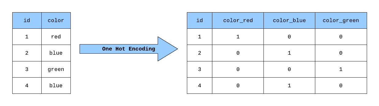
  |> Nx.stack(axis: 1)

> Build target tensor and hot-encode it > (https://projects.volkamerlab.org/teachopencadd/_images/OneHotEncoding_eg.png)

target_hot_encoded =
  target
  |> IO.inspect(label: "ORIGINAL TARGET")
  |> Scholar.Preprocessing.one_hot_encode(num_classes: 2)

> Build the Decision Tree and check its accuracy

model =
  EXGBoost.train(
    features,
    target_hot_encoded,
    obj: :binary_logistic,
    max_depth: 10
    # max_depth: 10
  )

predictions =
  EXGBoost.predict(model, features)
  |> Nx.argmax(axis: 1)
  |> dbg()

Scholar.Metrics.Classification.accuracy(target, predictions)

⚔️ Avoid overfitting with cross-validation

https://www.mathworks.com/discovery/overfitting/_jcr_content/mainParsys/image.adapt.full.medium.svg/1686825007300.svg

https://notes.club/elixir-nx/scholar/notebooks/cv_gradient_boosting_tree

alias Scholar.ModelSelection
alias Scholar.Preprocessing
alias Scholar.Metrics.Classification

## Utility functions

folding_fn = fn x -> ModelSelection.k_fold_split(x, 5) end

scoring_fn = fn x, y ->
  {x_train, x_test} = x
  {y_train, y_test} = y

  y_train_hot_encoded = Preprocessing.one_hot_encode(y_train, num_classes: 2)

  y_pred =
    EXGBoost.train(
      x_train,
      y_train_hot_encoded,
      obj: :binary_logistic,
      max_depth: 5,
      evals: [{x_train, y_train_hot_encoded, "training"}],
      verbose_eval: true
    )
    |> EXGBoost.predict(x_test)
    |> Nx.argmax(axis: 1)

  Classification.accuracy(y_test, y_pred)
end

## Compute the score

cv_scores =
  ModelSelection.cross_validate(
    features,
    target,
    folding_fn,
    scoring_fn
  )
  |> Nx.squeeze()

## Accuracy is the mean of the scores

Nx.mean(cv_scores)

🎨 Plot the Decision Tree

# # https://stackoverflow.com/questions/60186747/how-do-i-include-feature-names-in-the-plot-tree-function-from-the-xgboost-librar
# ["Pclass", "Age", "Sex", "SibSp", "Parch", "Fare", "Embarked"]
# |> Enum.with_index(fn element, index -> "#{index} #{element} q" end)
# |> Enum.join("\n")
# |> then(&File.write!("/Users/nicolo.gnudi/fmap.txt", &1))

# EXGBoost.Booster.get_dump(model, fmap: "/Users/nicolo.gnudi/fmap.txt", format: :json)
# |> Jason.Formatter.pretty_print()
# # |> then(& File.write!("/Users/nicolo.gnudi/dt.json", &1))

Export model and import it in Python for plotting

https://github.com/acalejos/exgboost/issues/29

# # Dump the model
# EXGBoost.write_weights(model, "/Users/nicolo.gnudi/dtw")

Then, install the required Python packages

pip3 install xgboost
pip3 install graphviz

And finally plot the Decision Tree

❯ python3

>>> import xgboost as xgb
>>> model = xgb.Booster()
>>> model.load_model("/Users/nicolo.gnudi/dtw.json")
>>> g = xgb.to_graphviz(model, fmap="/Users/nicolo.gnudi/fmap.txt")
>>> g.render(filename="/Users/nicolo.gnudi/dtg")
'/Users/nicolo.gnudi/dtg.pdf'

Take aways

Livebook is just a great tool
Playing with these data and ML libraries is a fun and rewarding experience
…and they might be useful in your daily job

Back