Drawing the Solar System

ex_astro =
  if File.exists?(Path.expand("../mix.exs", __DIR__)) do
    {:ex_astro, path: Path.expand("..", __DIR__)}
  else
    {:ex_astro, "~> 0.3"}
  end

Mix.install([ex_astro, {:kino, "~> 0.16"}])

Section

This notebook turns JPL ephemerides into SVG orbit diagrams using ex_astro. Everything astronomical in it — the time-scale conversions, the body states, the orbital elements — is a library call; the rest is plain Elixir and a bit of SVG.

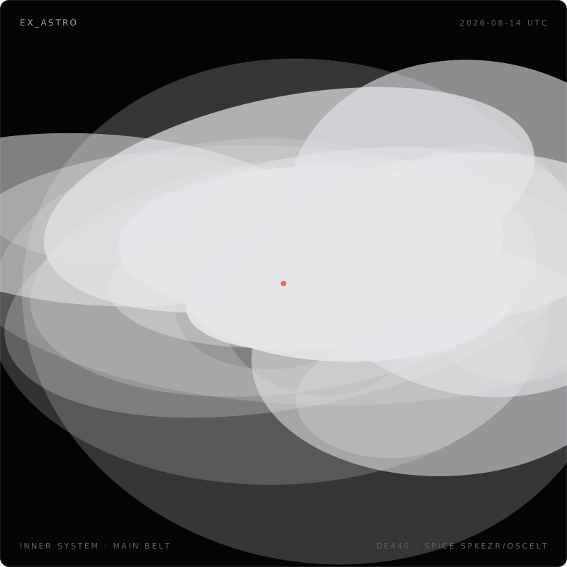
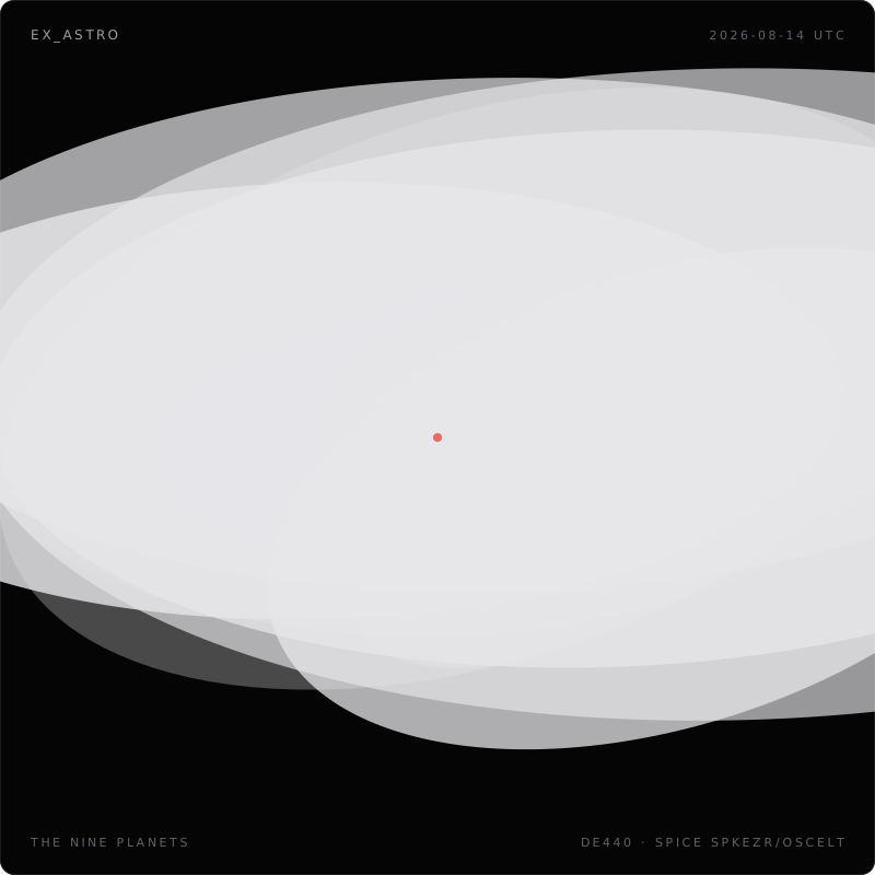
These are not artist’s impressions: every ellipse is the real osculating orbit of the body at the epoch, computed from the same DE440 ephemeris data that JPL uses. Eccentricities, inclinations, and node/periapsis orientations are true; the dots sit at the true positions and revolve with true period ratios.

The notebook is organised as a tutorial. The first half walks through the library: how a wall-clock time becomes ephemeris time, how a state vector becomes orbital elements, and what each Astro.Orbit function computes. The second half builds the diagrams in stages — first face-on, then through a tilted camera, then animated — so each drawing technique is visible on its own before they combine into the finished scenes.

The first evaluation downloads about 92 MB of SPICE kernels to ~/.cache/ex_astro/kernels (sha256-verified) and then writes solar-system.svg and inner-system.svg next to this notebook. The NIF build needs a C toolchain, liberfa, and libgmp at link time — inside this repo’s flake: nix develop, then open the notebook in Livebook.

Load kernels at runtime

SPICE reads everything — positions, masses, reference frames — from kernel files. This notebook needs four:

• de440s.bsp — an SPK (ephemeris) kernel: Chebyshev polynomials for the positions of the Sun, the planetary barycenters, and the Moon, 1849–2150
• gm_de440.tpc — a text PCK (constants) kernel: the gravitational parameter $GM$ of each of those bodies
• codes_300ast_20100725.bsp — an SPK with the 300 largest asteroids
• codes_300ast_20100725.tf — the frame definitions that asteroid SPK requires

The cell below streams missing files to disk with Req, verifies their sha256 digests, and loads each path through Astro.Kernel.

In a regular Mix project, mix astro.kernels downloads a useful default set into priv/kernels/; list the paths under config :ex_astro, :spice_kernels, [...] to load them when the application starts.

defmodule Orbits.Kernels do
  @moduledoc false

  @cache Path.expand("~/.cache/ex_astro/kernels")
  @naif "https://naif.jpl.nasa.gov/pub/naif/generic_kernels"
  @kernels [
    %{
      file: "de440s.bsp",
      url: "#{@naif}/spk/planets/de440s.bsp",
      sha256: "c1c7feeab882263fc493a9d5a5b2ddd71b54826cdf65d8d17a76126b260a49f2"
    },
    %{
      file: "gm_de440.tpc",
      url: "#{@naif}/pck/gm_de440.tpc",
      sha256: "924ddf4fb9ead9fe8a1aa55780bcabde40b09d00065d58226e24b68d8092f140"
    },
    %{
      file: "codes_300ast_20100725.tf",
      url: "#{@naif}/spk/asteroids/codes_300ast_20100725.tf",
      sha256: "15ee3b1731817774672725ccc226b249eb9ca5aa5d0a6a7805c91e5f57497f40"
    },
    %{
      file: "codes_300ast_20100725.bsp",
      url: "#{@naif}/spk/asteroids/codes_300ast_20100725.bsp",
      sha256: "7bb92faaadac29ec0b62aa96041a37c92ae24b9a5460de03d3fcaa2f63fe51f0"
    }
  ]

  def paths, do: Enum.map(@kernels, &Path.join(@cache, &1.file))

  def ensure_all do
    case Enum.reject(@kernels, &File.exists?(Path.join(@cache, &1.file))) do
      [] ->
        :ok

      missing ->
        File.mkdir_p!(@cache)
        Enum.each(missing, &download/1)
    end
  end

  # Stream to .tmp, verify status + sha256, then atomically rename.
  defp download(%{file: file, url: url, sha256: expected}) do
    path = Path.join(@cache, file)
    tmp = path <> ".tmp"
    IO.puts("downloading #{file} ...")

    try do
      response =
        Req.get!(url,
          into: File.stream!(tmp),
          raw: true,
          receive_timeout: 1_800_000,
          retry: false
        )

      response.status == 200 || raise "GET #{url} -> HTTP #{response.status}"
      verify!(tmp, file, expected)
      File.rename!(tmp, path)
    after
      File.rm(tmp)
    end
  end

  defp verify!(tmp, file, expected) do
    actual =
      tmp
      |> File.stream!(1_048_576)
      |> Enum.reduce(:crypto.hash_init(:sha256), &:crypto.hash_update(&2, &1))
      |> :crypto.hash_final()
      |> Base.encode16(case: :lower)

    actual == expected || raise "sha256 mismatch for #{file}: expected #{expected}, got #{actual}"
  end
end

Orbits.Kernels.ensure_all()
Enum.each(Orbits.Kernels.paths(), &(:ok = Astro.Kernel.load(&1)))
Astro.Kernel.loaded()

From a wall clock to ephemeris time

SPICE functions take ephemeris time (ET): TDB seconds past the J2000 epoch. Getting there from a UTC timestamp is a chain of three corrections, each with a physical reason:

• UTC → TAI — undo the leap seconds. TAI is what atomic clocks actually count; UTC is TAI plus an integer offset that changes when the IERS says so.
• TAI → TT — add the fixed 32.184 s. Terrestrial Time is the ideal clock on the geoid; the offset is historical, inherited from the old Ephemeris Time scale.
• TT → TDB — apply the relativistic periodic terms (< 2 ms). A clock at the solar-system barycenter ticks at a slightly different rate than one on Earth, modulated by Earth’s orbital motion.

Astro.Time.to_et/1 performs the whole chain. Internally it uses ERFA/SOFA two-part Julian Dates, which preserve sub-microsecond precision instead of collapsing the epoch into a single 64-bit float.

Every computation below is anchored to this one epoch.

epoch = ~U[2026-08-14 00:00:00Z]
et = Astro.Time.to_et(epoch)

A state vector from the ephemeris

Astro.Ephemeris.spkezr/5 returns the position and velocity of one body relative to another, in any SPICE reference frame. Bodies are named by NAIF ID strings ("10" = Sun, "3" = Earth-Moon barycenter, "2000001" = Ceres) or by name ("EARTH" works too — see Astro.Support.bodn2c/1).

The frame here is ECLIPJ2000 — the mean ecliptic of J2000, a frame frozen at the epoch, so the x-y plane is where Earth’s orbit lay in 2000 (the instantaneous orbital plane precesses slowly away from it). That is the natural canvas for a top-down solar-system drawing. "NONE" asks for the true geometric state; passing "LT+S" instead would give the apparent state, corrected for light travel time and stellar aberration.

One deliberate choice throughout this notebook: “Earth” is queried as "3", the Earth-Moon barycenter. The barycenter follows the smooth heliocentric orbit; Earth proper ("399") wobbles around it once a month, which would add a distracting ripple to the osculating elements.

# State of the Earth-Moon barycenter relative to the Sun, ecliptic frame,
# no aberration correction.
{:ok, [x, y, z, vx, vy, vz] = state, light_time} =
  Astro.Ephemeris.spkezr("3", et, "ECLIPJ2000", "NONE", "10")

%{
  position_km: {x, y, z},
  velocity_km_s: {vx, vy, vz},
  light_time_s: light_time
}

The osculating orbit

Six numbers — position and velocity — fully determine a two-body orbit. The conic that matches them at the epoch is called the osculating orbit (from Latin osculari, “to kiss”): it touches the real trajectory with the same position and velocity at that instant. If every perturbation — Jupiter’s pull, solar radiation pressure, relativity — switched off right now, this is the ellipse the body would coast on forever. Because the perturbations don’t switch off, the elements drift slowly, which is why they carry their epoch t0 with them.

Astro.Orbit.osculating/4 looks up the state (the same spkezr call as above), reads the observer’s gravitational parameter from the loaded PCK, and converts with SPICE’s oscelt. The struct fields follow SPICE’s element order:

Two of these deserve a note. SPICE stores the periapsis radius rather than the semi-major axis because $r_p$ stays finite and meaningful for parabolic and hyperbolic orbits, where $a$ diverges or goes negative. And $\mu = GM$ is kept as a single product because that is what orbits actually measure — $G$ and $M$ are each known far less precisely than their product.

{:ok, mu} = Astro.Support.gm(10)
{:ok, earth} = Astro.Orbit.osculating("3", "10", et, frame: "ECLIPJ2000", mu: mu)

Shape: semi-major axis and the apsides

The scalar shape of the ellipse follows from rp and ecc alone. The periapsis and apoapsis distances of an ellipse with semi-major axis $a$ are $r_p = a(1-e)$ and $r_a = a(1+e)$, so:

$$ a = \frac{r_p}{1-e}, \qquad r_a = r_p\,\frac{1+e}{1-e}, \qquad b = a\sqrt{1-e^2} $$

which is exactly what Astro.Orbit.semi_major_axis/1, periapsis/1, and apoapsis/1 return (the semi-minor axis $b$ we compute inline — it falls out of the drawing equation later). For Earth the numbers should look familiar: $a \approx 1$ au, perihelion just under, aphelion just over.

au_km = 149_597_870.7
a = Astro.Orbit.semi_major_axis(earth)

%{
  semi_major_axis_au: a / au_km,
  semi_minor_axis_au: a * :math.sqrt(1.0 - earth.ecc * earth.ecc) / au_km,
  perihelion_au: Astro.Orbit.periapsis(earth) / au_km,
  aphelion_au: Astro.Orbit.apoapsis(earth) / au_km,
  eccentricity: earth.ecc
}

Time: mean motion and the three anomalies

Where the body sits on the ellipse at a given time is the classic Kepler problem, and it involves three different angles (“anomalies”), each earning its keep:

• Mean anomaly $M$ — a fictitious angle that grows linearly with time. Trivial to propagate, but points nowhere physical.
• Eccentric anomaly $E$ — the angle in the ellipse’s auxiliary circle parametrization. This is the geometric one: it will drive the drawing.
• True anomaly $\nu$ — the actual angle from periapsis to the body, as seen from the focus. This is where the body physically is.

The mean motion comes from Kepler’s third law, and the mean anomaly is then just linear extrapolation from the epoch — Astro.Orbit.mean_motion/1 and mean_anomaly_at/2:

$$ n = \sqrt{\frac{\mu}{a^3}}, \qquad T = \frac{2\pi}{n}, \qquad M(t) = M_0 + n\,(t - t_0) $$

Getting from $M$ to $E$ means inverting Kepler’s equation,

$$M = E - e \sin E$$

which has no closed-form solution — centuries of iteration schemes started with this equation. Astro.Orbit.eccentric_anomaly/2 uses Newton’s method,

$$E_{k+1} = E_k + \frac{M - (E_k - e\sin E_k)}{1 - e\cos E_k}$$

starting from $E_0 = M + e\sin M$ and iterating to $10^{-13}$ rad — for planetary eccentricities that converges in a handful of steps. The last hop to the physical angle is closed-form, true_anomaly/2:

$$\tan\frac{\nu}{2} = \sqrt{\frac{1+e}{1-e}}\,\tan\frac{E}{2}$$

Mars, with $e \approx 0.09$, shows the three anomalies visibly disagreeing (all three coincide only at the apsides). The residual of Kepler’s equation confirms the solver:

{:ok, mars} = Astro.Orbit.osculating("4", "10", et, frame: "ECLIPJ2000", mu: mu)

deg = 180.0 / :math.pi()
mean = Astro.Orbit.mean_anomaly_at(mars, et)
ecc_anom = Astro.Orbit.eccentric_anomaly_at(mars, et)
true_anom = Astro.Orbit.true_anomaly_at(mars, et)

%{
  period_days: Astro.Orbit.period(mars) / 86_400,
  mean_motion_deg_day: Astro.Orbit.mean_motion(mars) * 86_400 * deg,
  mean_anomaly_deg: mean * deg,
  eccentric_anomaly_deg: ecc_anom * deg,
  true_anomaly_deg: true_anom * deg,
  kepler_residual_rad: ecc_anom - mars.ecc * :math.sin(ecc_anom) - mean
}

Closing the loop: elements back to a state

Astro.Orbit.state_at/2 propagates an orbit to any epoch and returns the Cartesian state (SPICE’s conics under the hood). Evaluated at the orbit’s own epoch it must reproduce the state vector the elements came from — a round-trip through the entire element machinery. The agreement is at the numerical-noise level: sub-millimeter over a distance of 1 au.

{:ok, [x2, y2, z2, vx2, vy2, vz2]} = Astro.Orbit.state_at(earth, et)

%{
  position_error_km: :math.sqrt((x2 - x) ** 2 + (y2 - y) ** 2 + (z2 - z) ** 2),
  velocity_error_km_s: :math.sqrt((vx2 - vx) ** 2 + (vy2 - vy) ** 2 + (vz2 - vz) ** 2)
}

Orientation: the perifocal basis

Shape and timing live inside the orbital plane; the three remaining elements ($\Omega$, $i$, $\omega$) say how that plane sits in space. They are the classic 3-1-3 Euler rotation: rotate by $\Omega$ about the frame’s z-axis to point at the ascending node, tilt by $i$ about that node line, then rotate by $\omega$ within the plane to point at periapsis.

Astro.Orbit.perifocal_basis/1 multiplies the three rotations out and returns the resulting orthonormal triad:

• $\hat u$ — unit vector toward periapsis
• $\hat v$ — 90° ahead of $\hat u$ in the orbital plane, along the direction of motion at periapsis
• $\hat w = \hat u \times \hat v$ — the orbit normal

The checks below confirm the triad is orthonormal and that the normal’s z-component equals $\cos i$ — the orbit normal makes exactly the inclination angle with the ecliptic pole. (One caveat worth knowing: for orbits with near-zero inclination — Earth in an ecliptic frame — the node direction is nearly degenerate, so $\Omega$ and $\omega$ individually become ill-defined while their sum, and the basis vectors themselves, stay perfectly good. Mars is inclined enough to be safely away from that.)

{u, v, w} = Astro.Orbit.perifocal_basis(mars)
dot3 = fn {ax, ay, az}, {bx, by, bz} -> ax * bx + ay * by + az * bz end

%{
  u: u,
  v: v,
  w: w,
  u_dot_v: dot3.(u, v),
  u_norm: :math.sqrt(dot3.(u, u)),
  w_z: elem(w, 2),
  cos_inc: :math.cos(mars.inc)
}

From orbit to picture: one ellipse, one matrix

Everything the diagrams need is now in hand, and it meets in a single equation. The position on an elliptic orbit, written in the perifocal basis and parametrized by eccentric anomaly, is:

$$ \vec r(E) = a(\cos E - e)\,\hat u + a\sqrt{1-e^2}\,\sin E\,\hat v $$

The $\cos E$ / $\sin E$ pair traces the auxiliary circle, $\sqrt{1-e^2}$ squashes it into an ellipse of semi-minor axis $b$, and the $-ae$ term slides the whole thing so that the focus — the Sun — sits at the origin, not the ellipse’s center.

Now apply any linear map $P$ to it — a rotation, an orthographic camera projection, a scaling, or all of them composed. Linear maps distribute over the sum:

$$ P(\vec r) = \vec c + \vec p\cos E + \vec q\sin E, \qquad \vec p = a\,P(\hat u),\quad \vec q = b\,P(\hat v),\quad \vec c = -ae\,P(\hat u) $$

That is precisely what SVG’s matrix(px py qx qy cx cy) transform does to a point $(\cos E, \sin E)$ on the unit circle. So each orbit in the diagram is literally <circle r="1"/> under one matrix() — the projected ellipse is exact, not approximated by line segments. And placing a dot at angle $E$ on the unit circle lands it exactly at the body’s projected position, because $E$ is the circle-parametrization angle. The eccentric anomaly earns its keep twice: once for Kepler timing, once as the drawing parameter.

Two SVG details make this practical:

• vector-effect="non-scaling-stroke" keeps stroke widths in screen pixels. Without it the matrix would scale strokes anisotropically and every ring would render thicker along its major axis.
• Each body dot is a zero-length path (M x y l .0001 0) with a round linecap, so its on-screen size is just its stroke width — immune to the ellipse matrix for the same reason.

The Orbits.Body module below reduces one body to exactly the drawing inputs the equation asks for: $a$ (in au), $e$, $\hat u$, $\hat v$, plus the period and current eccentric anomaly for the later stages. Orbits.Style holds the hand-tuned cosmetics — rings and dots fade with distance so fourteen orbits stay readable on one canvas.

defmodule Orbits.Style do
  @moduledoc false

  # name => {ring opacity, dot stroke width, dot opacity, trail degrees}
  @style %{
    mercury: {0.50, 3.0, 0.90, 50},
    venus: {0.45, 4.5, 0.90, 45},
    earth: {0.45, 4.5, 0.90, 45},
    mars: {0.40, 3.5, 0.85, 45},
    jupiter: {0.32, 7.0, 0.80, 35},
    saturn: {0.28, 6.5, 0.75, 35},
    uranus: {0.24, 5.0, 0.70, 30},
    neptune: {0.22, 5.0, 0.65, 30},
    pluto: {0.30, 2.5, 0.75, 30},
    ceres: {0.26, 2.5, 0.70, 25},
    pallas: {0.22, 2.0, 0.60, 25},
    juno: {0.20, 2.0, 0.55, 25},
    vesta: {0.24, 2.2, 0.65, 25},
    hygiea: {0.20, 2.0, 0.55, 25}
  }

  def get(name) do
    {ring_op, dot_w, dot_op, trail_deg} = Map.fetch!(@style, name)
    %{ring_op: ring_op, dot_w: dot_w, dot_op: dot_op, trail_deg: trail_deg}
  end
end

defmodule Orbits.Body do
  @moduledoc false

  @au_km 149_597_870.7

  # Reduce one sun-centered body to the drawing inputs: a, e, u-hat, v-hat,
  # plus period and current eccentric anomaly for the animation stage.
  def fetch({id, name}, et, mu) do
    {:ok, orb} = Astro.Orbit.osculating(id, "10", et, frame: "ECLIPJ2000", mu: mu)
    {u, v, _w} = Astro.Orbit.perifocal_basis(orb)

    Map.merge(Orbits.Style.get(name), %{
      name: name,
      a_au: Astro.Orbit.semi_major_axis(orb) / @au_km,
      e: orb.ecc,
      inc: orb.inc,
      period_s: Astro.Orbit.period(orb),
      ecc_anomaly: Astro.Orbit.eccentric_anomaly_at(orb, et),
      u: u,
      v: v
    })
  end
end

The camera is an orthographic projection: rotate the scene about the ecliptic pole by rotation (purely cosmetic — it keeps node lines from aligning with the canvas axes), tilt it by tilt away from face-on, and drop the depth coordinate. The y-sign flips because SVG’s y-axis points down. place/4 evaluates the boxed equation — $\vec p$, $\vec q$, $\vec c$ from $P(\hat u)$ and $P(\hat v)$ — and fit/2 uniformly rescales a whole scene so its widest orbit meets the canvas margin. (The compress argument is explained with the finished scenes; the default 1.0 means true scale.)

defmodule Orbits.Camera do
  @moduledoc false

  # Orthographic camera: scene rotation about the ecliptic pole, camera tilt
  # from face-on, then drop depth. The y flip converts to SVG's downward y.
  def project({x, y, z}, rotation, tilt) do
    x1 = x * :math.cos(rotation) - y * :math.sin(rotation)
    y1 = x * :math.sin(rotation) + y * :math.cos(rotation)
    {x1, -(y1 * :math.cos(tilt) - z * :math.sin(tilt))}
  end

  # The ellipse-as-unit-circle map: p = a P(u), q = b P(v), c = -ae P(u).
  # compress != 1.0 rescales each conic uniformly (r ~ a^compress), which
  # preserves e, i, and orientation — only relative sizes change.
  def place(body, rotation, tilt, compress \\ 1.0) do
    a = :math.pow(body.a_au, compress)
    b = a * :math.sqrt(1.0 - body.e * body.e)
    pu = project(body.u, rotation, tilt)
    pv = project(body.v, rotation, tilt)

    Map.merge(body, %{
      p: scale(pu, a),
      q: scale(pv, b),
      c: scale(pu, -a * body.e)
    })
  end

  # Uniform scene scale so the widest projected orbit touches the margin.
  def fit(orbits, extent) do
    s = extent / max_extent(orbits)
    Enum.map(orbits, &%{&1 | p: scale(&1.p, s), q: scale(&1.q, s), c: scale(&1.c, s)})
  end

  defp max_extent(orbits) do
    for %{p: {px, py}, q: {qx, qy}, c: {cx, cy}} <- orbits,
        t <- 0..719,
        reduce: 0.0 do
      acc ->
        th = t * :math.pi() / 360.0
        x = cx + px * :math.cos(th) + qx * :math.sin(th)
        y = cy + py * :math.cos(th) + qy * :math.sin(th)
        max(acc, max(abs(x), abs(y)))
    end
  end

  defp scale({x, y}, s), do: {x * s, y * s}
end

The renderer turns placed orbits into the SVG document: one matrix()-transformed group per body containing the unit-circle ring and the dot, plus the frame, labels, and an accessibility <desc>. The animation machinery it emits is the subject of stage 3; with animate: false it draws a static snapshot.

defmodule Orbits.Render do
  @moduledoc false

  @reference_anim_s 12.0
  @trail_step_deg 5
  @font "ui-monospace, 'JetBrains Mono', 'Fira Code', monospace"

  def scene(orbits, opts) do
    title = Keyword.fetch!(opts, :title)
    epoch = Keyword.fetch!(opts, :epoch)
    animate? = Keyword.get(opts, :animate, true)
    desc = Keyword.get(opts, :desc, default_desc(title, epoch))
    parts = Enum.map_join(orbits, "\n", &body_svg(&1, orbits, animate?))

    """
    <svg xmlns="http://www.w3.org/2000/svg" width="800" height="800" viewBox="0 0 800 800" role="img" aria-label="#{title}">
      <desc>
    #{indent(desc)}
      </desc>
      <rect x="0.5" y="0.5" width="799" height="799" rx="12" fill="#050505" stroke="#1c1c1f"/>
      <g transform="translate(400 400)" fill="none" stroke="#e6e6e9" stroke-width="1">
    #{parts}
<!-- sun -->

        <circle r="4" fill="#e25d52" stroke="none" opacity="0.9"/>
      </g>
      <g font-family="#{@font}" font-size="11" letter-spacing="2.5" fill="#606069">
        <text x="28" y="36" fill="#9d9da6" font-size="12">EX_ASTRO</text>
        <text x="772" y="36" text-anchor="end">#{Calendar.strftime(epoch, "%Y-%m-%d")} UTC</text>
        <text x="28" y="774">#{title}</text>
        <text x="772" y="774" text-anchor="end">DE440 \u00b7 SPICE SPKEZR/OSCELT</text>
      </g>
    </svg>
    """
  end

  defp body_svg(o, orbits, true) do
    """
<!-- #{o.name}: T = #{f(o.period_s / 86_400 / 365.25, 2)} y -->

        <g transform="#{matrix(o)}">
          #{ring(o)}
          <g>
            <animateTransform attributeName="transform" type="rotate" from="0" to="360" dur="#{anim_period(orbits, o)}s" repeatCount="indefinite"/>
            #{trail(o)}
            #{dot(o)}
          </g>
        </g>\
    """
  end

  defp body_svg(o, _orbits, false) do
    """
<!-- #{o.name}: T = #{f(o.period_s / 86_400 / 365.25, 2)} y -->

        <g transform="#{matrix(o)}">
          #{ring(o)}
          #{dot(o)}
        </g>\
    """
  end

  # The ellipse-as-unit-circle trick: matrix(px py qx qy cx cy) maps the
  # point (cos E, sin E) to c + p cos E + q sin E — the projected orbit.
  defp matrix(%{p: {px, py}, q: {qx, qy}, c: {cx, cy}}) do
    values = Enum.map_join([px, py, qx, qy, cx, cy], " ", &f(&1, 2))
    "matrix(#{values})"
  end

  defp ring(%{ring_op: op}) do
    ~s(<circle r="1" stroke-opacity="#{f(op, 2)}" vector-effect="non-scaling-stroke"/>)
  end

  # A zero-length round-capped path: dot size = stroke width, in screen px.
  defp dot(%{ecc_anomaly: ea, dot_w: w, dot_op: op}) do
    ~s(<path d="M #{f(:math.cos(ea), 4)} #{f(:math.sin(ea), 4)} l .0001 0" ) <>
      ~s(stroke-width="#{f(w, 1)}" stroke-linecap="round" stroke-opacity="#{f(op, 2)}" ) <>
      ~s(vector-effect="non-scaling-stroke"/>)
  end

  # A short arc of eccentric anomaly trailing behind the dot.
  defp trail(%{ecc_anomaly: ea, trail_deg: deg, ring_op: op}) do
    points =
      deg..0//-@trail_step_deg
      |> Enum.map(fn d -> ea - d * :math.pi() / 180.0 end)
      |> Enum.map_join(" L ", fn th -> "#{f(:math.cos(th), 4)} #{f(:math.sin(th), 4)}" end)

    ~s(<path d="M #{points}" stroke-opacity="#{f(op + 0.05, 2)}" stroke-linecap="round" ) <>
      ~s(vector-effect="non-scaling-stroke"/>)
  end

  # The fastest body revolves once per @reference_anim_s; everything else
  # scales by its true period ratio.
  defp anim_period(orbits, %{period_s: t}) do
    %{period_s: fastest} = Enum.min_by(orbits, & &1.period_s)
    f(@reference_anim_s * t / fastest, 1)
  end

  defp default_desc(title, epoch) do
    "#{title} at #{epoch} — generated by examples/orbits.livemd; do not edit by hand."
  end

  defp indent(desc) do
    desc
    |> String.trim_trailing()
    |> String.split("\n")
    |> Enum.map_join("\n", &("    " <> &1))
  end

  # Compact float formatting: fixed decimals, then strip trailing zeros.
  defp f(value, decimals) do
    value
    |> :erlang.float_to_binary(decimals: decimals)
    |> String.trim_trailing("0")
    |> String.trim_trailing(".")
    |> case do
      "-0" -> "0"
      s -> s
    end
  end
end

Stage 1: the face-on view

The simplest camera looks straight down the ecliptic pole: rotation 0, tilt 0, so the projection is just $(x, y, z) \mapsto (x, -y)$ and the drawing is a true top-down map of the inner system.

Worth spotting in the result: Mercury’s ring is visibly off-center. Its eccentricity is 0.206, so the Sun — sitting at the focus — is offset from the ellipse’s center by $ae \approx 0.08$ au. That offset is the $\vec c$ term of the matrix, straight from the ephemeris. The inclinations, on the other hand, are almost invisible from here: face-on, an inclined orbit just shrinks by $\cos i$ along one axis, a sub-percent effect even for Mercury’s 7°.

rocky = [{"1", :mercury}, {"2", :venus}, {"3", :earth}, {"4", :mars}]
bodies = Enum.map(rocky, &Orbits.Body.fetch(&1, et, mu))

face_on =
  bodies
  |> Enum.map(&Orbits.Camera.place(&1, 0.0, 0.0))
  |> Orbits.Camera.fit(330.0)
  |> Orbits.Render.scene(
    title: "INNER SYSTEM \u00b7 FACE-ON",
    epoch: epoch,
    animate: false
  )

Kino.HTML.new(face_on)

Stage 2: tilting the camera

A face-on map is honest but flat. Tilting the camera away from the pole turns the scene into the classic “textbook solar system” perspective — and because the projection is still linear, the tilted orbits are still exact ellipses drawn by the same unit-circle trick, just with different $\vec p$, $\vec q$, $\vec c$.

The finished scenes use two fixed angles: the scene rotated 15° about the pole (cosmetics: nothing interesting should line up with the canvas axes) and the camera tilted 66° from face-on — enough foreshortening to read as 3D, not so much that the inner orbits collapse into the Sun. Tilting is also what finally makes inclination visible: an inclined orbit’s out-of-plane excursion now leaks into the vertical screen axis, which is why Mercury’s ring starts to stand apart from the others below (and why Pallas, inclined almost 35°, cuts so dramatically across the finished belt scene).

Each tab re-fits the scene to the canvas, so the tilted views aren’t merely squashed — they’re re-scaled to fill the frame.

rad = :math.pi() / 180.0

tilted = fn tilt_deg ->
  bodies
  |> Enum.map(&Orbits.Camera.place(&1, 15.0 * rad, tilt_deg * rad))
  |> Orbits.Camera.fit(330.0)
  |> Orbits.Render.scene(
    title: "INNER SYSTEM \u00b7 TILT #{tilt_deg}\u00b0",
    epoch: epoch,
    animate: false
  )
end

Kino.Layout.tabs(
  "Face-on": Kino.HTML.new(tilted.(0)),
  "Tilted 33°": Kino.HTML.new(tilted.(33)),
  "Tilted 66°": Kino.HTML.new(tilted.(66))
)

Stage 3: setting it in motion

Animation falls out of the geometry for free. The dot sits at angle $E$ on the unit circle inside the matrix group — so rotating the unit circle underneath the matrix sweeps the dot along the true projected ellipse. One SMIL <animateTransform type="rotate"> per body does it, no JavaScript, and it keeps playing inside <img> tags and GitHub’s image proxy, where scripts are stripped.

Each body starts at its true eccentric anomaly at the epoch and revolves with its true period ratio: the fastest body (Mercury) takes 12 s per revolution and everything else scales by $T / T_{\text{fastest}}$. The faint trail is a short arc of $E$ drawn behind the dot, inside the same rotating group.

One honest limitation: SMIL rotates at a constant rate, i.e. uniformly in $E$, while Kepler timing has $\dot E = n / (1 - e\cos E)$ — bodies really sweep faster near perihelion. The path and the period are exact; the rate is off by up to $\pm e$ (Kepler’s equation bounds the angular offset by $|E - M| \le e$, so the dot leads or lags its true position by at most $e/2\pi$ of a revolution — 0.3% for Earth, 3.3% for Mercury). An <animate keyTimes> spline could fix even that, at the cost of readability — for a diagram, uniform $E$ is the right trade.

animated =
  bodies
  |> Enum.map(&Orbits.Camera.place(&1, 15.0 * rad, 66.0 * rad))
  |> Orbits.Camera.fit(330.0)
  |> Orbits.Render.scene(
    title: "INNER SYSTEM \u00b7 ANIMATED",
    epoch: epoch,
    animate: true
  )

Kino.HTML.new(animated)

The finished scenes

The two committed diagrams are just the pipeline above with body lists and one extra idea each:

• The nine planets — all planets plus Pluto. At true scale this is hopeless: Pluto’s semi-major axis is about 100× Mercury’s, so the inner system would vanish into a few pixels. Instead each conic is uniformly rescaled to $r \sim a^{0.4}$, which compresses the ratio to about 6.3×. Because the rescaling is uniform per orbit, every eccentricity, inclination, and orientation stays true — only the relative sizes lie, and the <desc> says so.
• Inner system + main belt — the rocky planets and the five largest main-belt asteroids (from the CODES asteroid kernel), at true scale (compress: 1.0). Watch Pallas: its 35° inclination is the most dramatic out-of-plane excursion in either scene.

Each SVG embeds its full provenance in the <desc> — sources, frame, projection — so the files stand alone once they leave the repo.

defmodule Orbits.Scenes do
  @moduledoc false

  @out __DIR__

  # NAIF ID strings: planets by barycenter ID, asteroids by 2000000 + IAU number
  @inner [{"1", :mercury}, {"2", :venus}, {"3", :earth}, {"4", :mars}]
  @outer [{"5", :jupiter}, {"6", :saturn}, {"7", :uranus}, {"8", :neptune}, {"9", :pluto}]
  @belt [
    {"2000001", :ceres},
    {"2000002", :pallas},
    {"2000003", :juno},
    {"2000004", :vesta},
    {"2000010", :hygiea}
  ]

  @scenes [
    %{
      file: "solar-system.svg",
      title: "THE NINE PLANETS",
      compress: 0.4,
      bodies: @inner ++ @outer
    },
    %{
      file: "inner-system.svg",
      title: "INNER SYSTEM \u00b7 MAIN BELT",
      compress: 1.0,
      bodies: @inner ++ @belt
    }
  ]

  @psi 15.0 * :math.pi() / 180.0
  @tilt 66.0 * :math.pi() / 180.0
  @fit_extent 330.0

  def run(et, epoch, mu) do
    Enum.map(@scenes, &render(&1, et, epoch, mu))
  end

  defp render(scene, et, epoch, mu) do
    orbits =
      scene.bodies
      |> Enum.map(&Orbits.Body.fetch(&1, et, mu))
      |> Enum.map(&Orbits.Camera.place(&1, @psi, @tilt, scene.compress))
      |> Orbits.Camera.fit(@fit_extent)

    svg =
      Orbits.Render.scene(orbits,
        title: scene.title,
        epoch: epoch,
        desc: desc(scene, epoch)
      )

    path = Path.join(@out, scene.file)
    File.write!(path, svg)

    %{file: scene.file, path: path, title: scene.title, svg: svg, orbits: orbits}
  end

  defp desc(%{title: title, compress: k}, epoch) do
    """
    #{title} at #{epoch} — real osculating orbits from JPL ephemerides
    (DE440s planets, gm_de440 GM constants, CODES codes_300ast asteroids;
    https://naif.jpl.nasa.gov/pub/naif/generic_kernels/) through the
    ex_astro library (SPICE spkezr + oscelt, sun-centered, ECLIPJ2000
    frame). Each orbit is the osculating conic at the epoch,
    orthographically projected (scene rotated 15 deg, camera tilted 66 deg
    from face-on) and drawn as a unit circle under a matrix() transform.
    Eccentricities, inclinations and node/periapsis orientations are true;
    #{scale_note(k)} Body dots start at their true eccentric anomalies and
    revolve with true period ratios.
    Generated by examples/orbits.livemd — do not edit by hand.
    """
  end

  defp scale_note(1.0), do: "radial distances are to scale (r ~ a)."
  defp scale_note(k), do: "radial distances are compressed (r ~ a^#{k})."
end

[solar, inner] = Orbits.Scenes.run(et, epoch, mu)

The same osculating elements that went into the ellipses:

defmodule Orbits.Table do
  def rows(orbits) do
    deg = 180.0 / :math.pi()

    Enum.map(orbits, fn o ->
      %{
        body: o.name,
        a_au: Float.round(o.a_au, 4),
        e: Float.round(o.e, 4),
        i_deg: Float.round(o.inc * deg, 2),
        e0_deg: Float.round(o.ecc_anomaly * deg, 1),
        period_days: Float.round(o.period_s / 86_400, 1)
      }
    end)
  end
end

Kino.Layout.tabs(
  "Inner system": Kino.DataTable.new(Orbits.Table.rows(inner.orbits)),
  "Nine planets": Kino.DataTable.new(Orbits.Table.rows(solar.orbits))
)

And the diagrams themselves, written next to this notebook:

Kino.Layout.tabs(
  "Inner system": Kino.HTML.new(inner.svg),
  "Nine planets": Kino.HTML.new(solar.svg)
)

%{inner: inner.path, solar: solar.path}

Going further

The same pattern scales to any body pair the loaded kernels cover:

• Moon systems — load jup365.bsp or sat441.bsp and center scenes on "599" (Jupiter) or "699" (Saturn) to draw the Galilean or Saturnian moons. Both kernels are in the mix astro.kernels default set.
• Spacecraft-style geometry — pass "LT+S" instead of "NONE" to get apparent (light-time and stellar-aberration corrected) states as seen by the observer.
• Positions over time — call spkezr/5 in a loop over et values to trace trajectories instead of osculating snapshots.