Introduction to Integrator

Mix.install([
  {:integrator, github: "woodward/integrator"},
  {:kino_vega_lite, "~> 0.1"}
])

Numerical Integration in Elixir

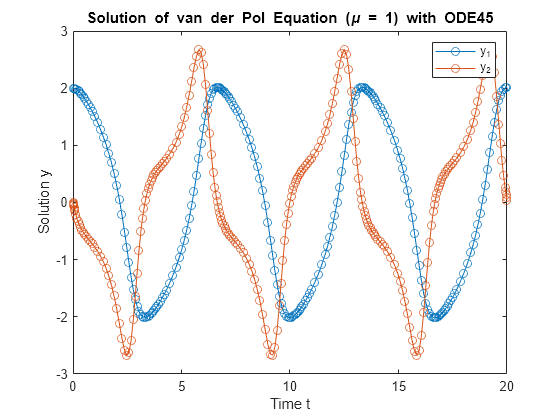
Numerical integration is easy with Integrator. For example, let’s integrate the Van der Pol equation Integrator.SampleEqns.van_der_pol_fn for 20 seconds:

alias Integrator.DataCollector
alias Integrator.Point
alias Integrator.SampleEqns

t_initial = Nx.f64(0.0)
t_final = Nx.f64(20.0)
x_initial = Nx.f64([2.0, 0.0])

{:ok, pid} = DataCollector.start_link()
output_fn = &DataCollector.add_data(pid, &1)

opts = [type: :f64, output_fn: output_fn]
Integrator.integrate(&SampleEqns.van_der_pol_fn/2, t_initial, t_final, x_initial, opts)

Now you can plot the results via Kino:

alias VegaLite, as: VL

data =
  DataCollector.get_data(pid)
  |> Enum.map(&Point.to_number(&1))
  |> Enum.map(fn point ->
    %{t: t, x: x} = point

    [
      %{t: t, x: List.first(x), x_value: "x[0]"},
      %{t: t, x: List.last(x), x_value: "x[1]"}
    ]
  end)
  |> List.flatten()

chart =
  VL.new(width: 600, height: 400, title: "Solution of van der Pol Equation (μ = 1) with Dormand-Prince45")
  |> VL.mark(:line, point: true, tooltip: true)
  |> VL.encode_field(:x, "t", type: :quantitative)
  |> VL.encode_field(:y, "x", type: :quantitative)
  |> VL.encode_field(:color, "x_value", type: :nominal)
  |> VL.data_from_values(data)
  |> Kino.VegaLite.new()
  |> Kino.render()

Compare this with the plot from the Matlab ode45 manual page: